Impact of Weather on Sydney Water Medium Term
Consumption Forecasts
Adrian Barker
July 3, 2017
1

---

Executive Summary
This document reports on an investigation conducted by the UNSW on a mathemati-
cal model used by Sydney Water to produce medium-term water consumption forecasts.
Precipitation, temperature and evaporation weather variables are included in the explana-
tory variables of the model. The primary focus of this investigation was to examine the
sensitivity of the model consumption forecasts to changes in the weather.
The model software together with a reduced data set was migrated to the UNSW
computing environment. This migration enabled much faster runs of the model, which
were needed for this investigation and provides a range of opportunities for the future.
Weather data for the model is taken from 12 weather stations and then spatially
interpolated to each property in the Sydney Water delivery system using a method known
as inverse distance weighting. A comparison is made between inverse distance weighting
and the spatial interpolation method used for the Australian Water Availability Project
(AWAP) gridded data set.
One hundred different weather scenarios for the financial years 2014/15 to 2024/25
were generated using a stochastic weather generator fitted from the AWAP gridded data
set. Consumption forecasts based on each of these weather scenarios were calculated
using the model. The average range of total consumption forecasts for a financial year
was 7.39%. Perturbations of these weather scenarios facilitated the estimation of the
effect on consumption forecasts of each weather variable at each weather station. An
increase in precipitation result in a decrease in forecast consumption, whereas an increase
in temperature or evaporation result in an increase in forecast consumption. The mag-
nitude of forecast consumption changes is similar for each of precipitation, temperature
and evaporation.
The model consumption forecasts agree well with actual consumption, though the
model tends to slightly underestimate the effect of weather. An examination was con-
ducted of the correlation between consumption and other weather variables based of cli-
mate extreme indices. It was found that each of the precipitation and temperature indices
used by the SWCM has a strong correlation with consumption. Several other indices were
2

---

also found to have a strong correlation with consumption. These indices may be useful
explanatory variables in any future consumption model.
We make the following recommendations and suggestions for future work.
• We suggest an exploration of alternative data – for example AWAP – to examine the
dependence of water use estimates on the 12 BoM weather stations used by Sydney
water;
• We suggest an exploration of the NSW/ACT regional climate modeling project
(NARCliM), including the generation of a set of projections, to assess the impact
of the underlying model assumptions on consumption forecasts.
• We suggest Sydney Water consider extending their modeling systems to use daily
data, replacing the use of quarterly weather and consumption data where possible;
• We suggest Sydney Water should consider a full review of SWCM including model
structure. This would enable other climate extremes indices to be examined for
their impact on water consumption.
3

---

1
Introduction
Sydney Water is a NSW State Government owned organisation which provides water to
almost five million people across Sydney, the Blue Mountains and the Illawarra (Figure
1). One of Sydney Water’s obligations is to provide a price submission every four years to
the Independent Pricing and Regulatory Tribunal (IPART) which includes the expected
income and expenses of Sydney Water operations.
For the 2014 submission to IPART, Sydney Water generated consumption forecasts
using a model which was originally developed as part of an investigation into the price
elasticity of water demand, (Abrams et al. (2012)). This model is hereafter referred to as
the Sydney Water consumption model (SWCM). Although weather was not the primary
focus of the SWCM, it was found that the weather variables precipitation, maximum
temperature and evaporation were statistically significant explanatory variables.
The University of New South Wales (UNSW) was engaged by Sydney Water to investi-
gate the skill of the SWCM in accounting for the impact of weather on water consumption.
This document is the report on that investigation.
2
Model Description
The SWCM is a dynamic panel data model, (Wooldridge (2010)). Panel data consists
of repeated observations on the same cross section of a population. For the SWCM, this
means repeated observations of water consumption on water consumers in the Sydney
Water network. For most consumers, a water consumption observation is the meter read-
ing taken each quarter prior to a water bill being generated. A dynamic panel data model
is one where past values of the response variable are included as explanatory variables.
The SWCM model equation for a residential property is
ln Ci,t = α ln Ci,t−1 + β0xi,t
(1)
4

---

Property Type
Total Number
Model Subset
Single Dwellings
1,052,960
127,209
Townhouse Units
100,757
99,761
Strata Units
421,571
133,187
Flats
116,168
111,003
Dual Occupancies
27,158
26,522
Table 1: List of residential property types with the total number of properties in the
Sydney Water region (June, 2014) and the number of those properties included in the
subset of properties used by the SWCM.
where α, β are model parameters, Ci,t is the consumption at property i during quarter t
and xi,t is a vector of explanatory variables.
For the purposes of the SWCM, water consumption is divided into residential and non-
residential consumption. Residential consumption consists of consumption by residential
properties which are categorised into the property types listed in Table 1. Consumption
is forecast for each of the residential properties analysed by the model and then summed
to produce a forecast for total residential consumption. Explanatory variables included in
the model which are used to explain residential consumption include: weather, historical
consumption, property type, participation in the WaterFix programme, possession of a
rain water tank, compliance with the Building Sustainability Index (BASIX), water price
and season.
The non-residential sector includes all property types not included in the residential
models. Non-residential properties were hierarchically segmented on the basis of con-
sumption levels, participation in water conservation programs and property types. The
first segment consists of the six highest water users. The second consists of all proper-
ties which participated in Every Drop Counts (EDC), Sydney Water’s water conservation
program for the non-residential sector. Finally, remaining properties were grouped in to
6 segments based on their property type classification. The resulting 8 segments are:
• Top 6 customers
• EDC participants
• Industrial
5

---

• Commercial
• Government and Institutional
• Agricultural
• Non-residential strata units
• Standpipes
A separate demand forecasting model was developed for each customer in the Top
6 segment. These models are generally based on historical average consumption with
allowances for planned water conservation activities. To forecast demand for the other
segments it is assumed that average demand will remain constant at the levels observed
in 2011/12, the last full year for which data was available at the time the non-residential
models were built. To correct the observed demand in 2011/12 for the impacts of above
or below average weather conditions, a combined seasonal-decomposition and time series
regression model of average demand was estimated.
Forecast property numbers are based on average growth rates. An important feature
of the non-residential sector is that property growth in the last 15 to 20 years is very
heavily concentrated in the segment of non-residential units and therefore forecast prop-
erty growth is heavily skewed towards units. The average consumption of this segment
is much lower than the average demand of the other segments. As a result, even though
average demand in each segment is assumed constant for forecasting purposes, overall
average demand by non-residential properties is forecast to decrease over time.
The weather variables used by the SWCM are listed in Table 2. The weather stations
used to provide weather variable data are listed in Table 3 and a map of these weather
stations is presented in Figure 1. Weather variables are aggregated to quarterly variables
when calculating residential consumption and to monthly variables when calculating non-
residential consumption. For each of the weather variables, long term averages are cal-
culated over the 30-year period 1980-2010. Generally, weather variables are included in
the SWCM as the difference between the current value and the long term average. The
model was fitted using data from 2010/11 to 2013/14. The last water restrictions for the
6

---

Abbreviation
Description
PRE
Average daily precipitation
GT2MM
Number of days when precipitation exceeds 2mm
TMAX
Average daily maximum temperature
GT30C
Number of days when maximum temperature exceeds 30◦C
EVAP
Average daily pan evaporation
Table 2: List of weather variables used by the SWCM.
Station Name
Station Id
PRE
GT2MM
TMAX
GT30C
EVAP
Albion Park
68241
Y
Y
Y
Y
N
Bellambi
68228
Y
Y
Y
Y
N
Camden
68192
Y
Y
Y
Y
N
Holsworthy
66161/67117
Y
Y
Y
Y
N
Katoomba
63039
Y
Y
Y
Y
N
Penrith
67113
Y
Y
Y
Y
N
Prospect
67019
Y
Y
Y
Y
Y
Richmond
67105/67021
Y
Y
Y
Y
Y
Riverview
66131
Y
N
Y
N
Y
Springwood
63077
Y
Y
Y
Y
N
Sydney Airport
66037
Y
Y
Y
Y
Y
Terrey Hills
66059
Y
Y
Y
Y
N
Table 3: Weather data provided by weather stations for the SWCM.
Sydney Region were lifted in June 2009. This last round of water restrictions appears to
have changed water use habits in the Sydney Region. Therefore, water consumption data
prior to 2009, at times when there were no water restrictions, were not used for model
fitting.
3
Software Migration to UNSW Environment
One of the early objectives of this investigation was to migrate the SWCM software onto
the UNSW environment in order to enable the calculation of consumption forecasts from a
large number of weather scenarios. A weather scenario refers to a single set of data for each
of the weather variables (Table 3) over the period covered by the financial years 2010/11
to 2024/25. The UNSW environment consists of a cluster of Linux servers connected to a
single Storage Area Network (SAN). Each of the Linux servers runs 16 CPUs with 256GB
of RAM.
Originally, the SWCM was implemented on a Windows PC using SPSS software (IBM
7

---

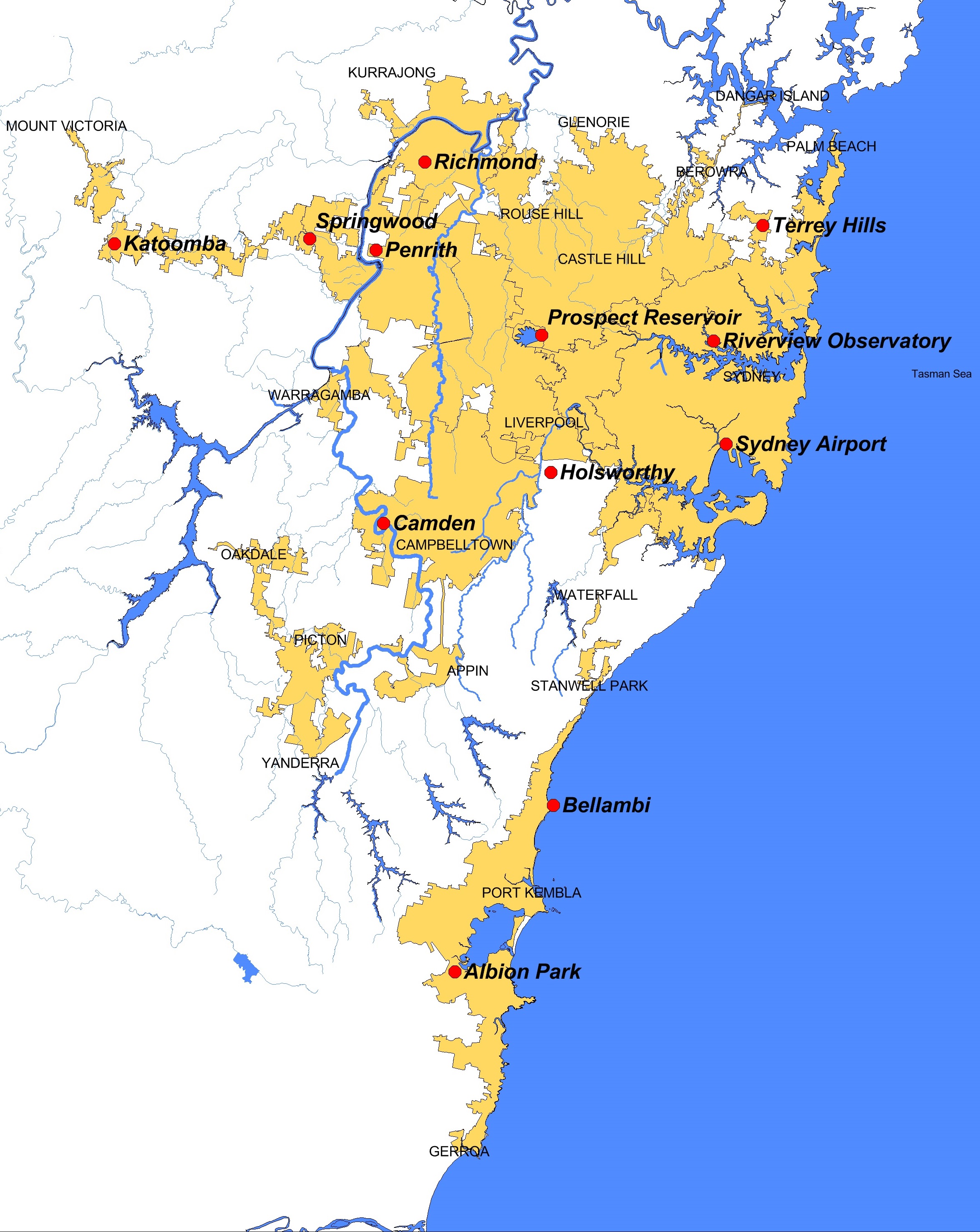
Figure 1: Sydney Water area of operations (orange) and location of the weather stations
(red) used by the SWCM, (Table 3).
8

---

(2017)) and it would take several hours to calculate consumption forecasts from a single
weather scenario. At the beginning of this investigation, Frank Spanninks (Sydney Water)
was able to reduce the SWCM run-times down to about 18 minutes per weather scenario,
by coding changes and by only calculating consumption forecasts for a representative
sample of the residential properties (Table 1).
SWCM was able to be migrated to run on the UNSW environment using SPSS soft-
ware. This migration required only minimal code changes and resulted in a run-time of
about 12 minutes. There is little capability in SPSS to utilise the parallel processing ca-
pacity of the UNSW enviroment, so it was decided to migrate the SWCM software from
SPSS to MATLAB (Mathworks (2017)). This migration required a substantial effort,
but was made easier by the presence of the SPSS version of SWCM which allowed the
comparison of intermediate and final results.
Once migrated to MATLAB, it was possible to run 10 weather scenarios in parallel
and run a total of 100 scenarios in about 110 minutes. Note that a migration of SWCM
to either R (R (2017)) or Python (Python (2017)) rather than MATLAB was also a
reasonable option which may have achieved even better results, but was not attempted.
While these technical changes to enable SWCM on a Linux cluster appear simply
a question of efficiency, they open up major new opportunities that we employ here.
Specifically, these technical changes enable hundreds of simulations to be conducted to
assess uncertainty and translate forecasts into probabilities.
4
Generation of Weather Scenarios
4.1
Introduction
The generation of large numbers of weather scenarios which are consistent with historical
observations is usually referred to as stochastic weather generation. Stochastic weather
generation has applications in many areas including agriculture, ecology and hydrology.
Reviews of the many different methods proposed can be found in Wilks and Wilby (1999),
Srikanthan and McMahon (2001) and Ailliot et al. (2015).
9

---

Weather scenarios which can be used by the SWCM need to contain monthly sequences
of the weather variables precipitation, number of days greater than 2mm, maximum tem-
perature, number days greater than 30◦C and evaporation at the weather stations listed
in Table 3. Initially, daily sequences of precipitation, maximum temperature and evapo-
ration are generated, from which it is straightforward to generate monthly sequences of
number of days greater than 2mm and number of days greater than 30◦C and also to
aggregate the daily sequences of precipitation, maximum temperature and evaporation
into monthly sequences. Following a similar approach to Richardson (1981), we consider
precipitation to be the primary variable, then condition maximum temperature on pre-
cipitation and finally condition evaporation on precipitation and maximum temperature.
The precipitation and maximum temperature data used to fit stochastic weather
models was the Australian Water Availability Project (AWAP) gridded data set (Jones
et al. (2009)). The AWAP data-set provides precipitation and temperature data on a
0.05◦ × 0.05◦ (approximately 5km) grid across Australia for the period 1910-2016. The
main advantage of using AWAP data rather than Bureau of Meteorology (BOM) data is
that there are no missing values. There is some loss of precision in using AWAP data
rather than BOM data, mainly for precipitation data, (Contractor et al. (2015)) though
this is less significant in the Sydney Region where there is a large number of BOM weather
stations. For this investigation, the AWAP data used was from the nearest grid point to
the BOM weather stations in Table 1 over the period (1960-2015). AWAP data prior to
1960 was not used due to the relative scarcity of weather stations in the Sydney Region
prior to 1960 (Jones et al. (2009)).
The evaporation data used to fit the stochastic weather models was the BOM data at
the weather stations listed in Table 1 over the period 2001-2010 for daily data and 2005-
2014 for yearly data. Daily evaporation data for which the quality was not confirmed or
which was accumulated over more than one day was not used. The evaporation data used
in this investigation was provided by Sydney Water.
Precipitation and evaporation data are recorded for the 24 hour period to 9am whereas
maximum temperature data are recorded for the 24 hour period from 9am. For the
10

---

purposes of this investigation, precipitation and evaporation data were shifted back 24
hours, so that all weather variables reflect the 24 hour period from 9am.
4.2
Precipitation
The daily precipitation model is a variation of the commonly used combination of oc-
currence and intensity models (Katz (1977)). In Katz (1977), occurrence is a binary
variable which indicates whether the day is ”wet” or ”dry”, i.e. whether precipitation
exceeds some small threshold, and intensity is the amount of precipitation which occurs
on a ”wet” day. Often, a first-order, two-state Markov chain is used for the occurrence
model and a gamma distribution is used for the intensity model. To address some of the
shortcomings found with these choices, various higher-order, multi-state Markov chains
with alternative intensity distributions have been proposed (Gregory et al. (1993), Jones
and Thornton (1993) and Suhaila and Jemain (2007)).
For the daily occurrence model, we chose a first-order eight-state Markov chain with
thresholds set at
Thresholds = (0mm, 1mm, 2mm, 4mm, 8mm, 15mm, 35mm) .
(2)
The threshold at 2mm was chosen to match the GT2MM weather variable in the SWCM
and improves the intersite correlation and the interannual variability of the GT2MM
weather variable. The other thresholds were chosen so that sufficient observed data ex-
ists between the thresholds. The addition of the other thresholds to create a eight-state
Markov chain improves the intersite correlation of the average precipitation weather vari-
able.
An individual daily occurrence model is fitted for each site and each month (144
models). The fitted model consists of an 8×8 transition probability matrix. The transition
probability from occurrence state i to occurrence state j is the conditional probability
P {Od = j|Od−1 = i} ,
(3)
11

---

Od−1Od
0
1
2
3
4
5
6
7
0
0.668
0.198
0.038
0.033
0.023
0.017
0.020
0.003
1
0.387
0.309
0.064
0.087
0.064
0.044
0.033
0.011
2
0.238
0.307
0.099
0.139
0.079
0.079
0.030
0.030
3
0.155
0.373
0.091
0.082
0.127
0.073
0.055
0.045
4
0.248
0.317
0.079
0.050
0.109
0.129
0.040
0.030
5
0.187
0.253
0.088
0.099
0.077
0.132
0.088
0.077
6
0.095
0.238
0.079
0.111
0.143
0.143
0.095
0.095
7
0.029
0.086
0.057
0.029
0.171
0.286
0.171
0.171
Table 4:
The transition probability matrix for Sydney Airport in January.
The
(i + 1, j + 1)th entry of the transition probability matrix is the conditional probability
that the occurrence state on day d, Od = (j) given that the occurrence state on day d − 1,
Od−1 = (i). The sum of the transition probabilities in each row equals one.
where Od is the occurrence state on day d. The occurrence state on day d is 0 if the pre-
cipitation on day d is zero, is 1 if the daily precipitation is greater than the first threshold
0mm and less than or equal to the second threshold 1mm, etc. The occurrence state on
day d is 7 if the precipitation on day d is greater than the seventh threshold, 35mm. An
example transition probability matrix is shown in Table 4. The transition probabilities in
Table 4 indicate that light precipitation days tend to follow light precipitation days and
heavy precipitation days tend to follow heavy precipitation days. This is typical of all
sites in the Sydney region and all months.
To generate a sequence of daily occurrence states {Os,d}, we first generate sequences of
independent, identically distributed (iid) standard Gaussian random variables, {us,d} for
each site s. Let T Ps,m (i, j) denote the (i + 1, j + 1)th entry of the transition probability
matrix for site s and month m. Given occurrence state Os,d−1 we set
(
j
)
X
Os,d = max Φ (us,d) <
T Ps,m (Os,d−1, j)
(4)
j
k=1
where Φ is the cumulative distribution function of the standard Gaussian distribution and
m is the month of day d. Initial values for the daily occurrence state sequences are set to
zero. The intersite correlation of the sequences {us,d} is estimated by simulation.
As with the daily occurrence model, an intensity distribution was estimated for each
site and each month, (144 distributions). A choice was made from the same set of dis-
12

---

tributions used in Suhaila and Jemain (2007), i.e. the exponential, gamma, Weibull and
their associated mixture distributions. In each case maximum likelihood estimation was
used. Two different measures for goodness of fit were used to compare the distributions.
The first goodness of fit measure is the integral of the absolute value of difference between
the fitted quantile function and the empirical quantile function,
Z
1 

Z


1 =
b
Qfit (p) − b
Qemp (p) dp
(5)


0
where b
Qfit (p) is the fitted quantile function and b
Qemp (p) is the empirical quantile function.
The second goodness of fit measure is the integral of the absolute value of difference
between the logs of the fitted quantile function and the empirical quantile function,
Z
1 




Z


2 =
ln
b
Qfit (p) − ln b
Qemp (p)
dp.
(6)


0
The Z1 goodness of fit measure tends to assess the fit only at high quantiles, whereas
Z2 more evenly assesses the fit across the entire distribution. For Z1, the mixed Weibull
distribution was the best fit for 92 of the site/month pairs, the mixed Gamma for 10 and
the Weibull for 42. For Z2, the mixed Weibull distribution was the best fit for 131 of the
site/month pairs and the mixed Gamma for 13. When the mixed Weibull distribution
was not the best fit it was second best on 56 occasions and third best on 9. These results
are largely in agreement with those reported in Suhaila and Jemain (2007). Thus, rather
than use different distributions for different site/month pairs it was decided to use the
mixed Weibull distribution to model daily intensity for all site/month pairs.
The density function for a mixed Weibull distribution is given by
 α 

 x α1
 α 

 x α2
f (x; ω, α
1
2
1, β1, α2, β2) = ω
exp −
+ (1 − ω)
exp −
(7)
β1
β1
β2
β2
where ω ∈ [0, 1] is the mixture parameter, α1, α2 > 0 are the shape parameters and
β1, β2 > 0 are the scale parameters.
A common problem in stochastic weather generation is the presence of a negative bias
13

---

in interannual variability (Gregory et al. (1993), Wilks (1999), Kysely and Dubrovsky
(2005)). The use of higher-order, multi-state Markov chains has been proposed as a
method to reduce the negative bias in interannual variability (Gregory et al. (1993)),
however the consequent increase in the number of model parameters can result in model-
fitting problems for small data sets. For this investigation, we use an alternative method,
where low frequency models (yearly) for the same weather variable are coupled with the
high frequency (daily) models (Wang and Nathan (2007)).
The low frequency precipitation model chosen is an autoregressive (AR) model (Brock-
well and Davis (1991)) on the number of ”wet” days per year,
GT0MMy,s = µs + φsGT0MMy−1,s + ey,s
(8)
where GT0MMy,s is the number of ”wet” days in year y at site s, {ey,s} is a sequence of iid
Gaussian random variables with distribution N 0, σ2  and µ
e,s
s, φs are model parameters.
The observed distribution of the yearly GT0MM for each site is reasonably symmetrical
with a lighter tail than the Gaussian distribution. The minimum and maximum number
of ”wet” days recorded in AWAP data (1960-2015) for any of the 12 weather stations listed
in Table 3 is 101 and 253 respectively. Therefore, the boundary problems where there
are close to 0 ”wet” days or close to 365 ”wet” days, which may occur when using this
method to model in either very arid or very wet locations are not relevant when modelling
in the Sydney Region. The correlation between the innovation sequences,{ey,s}, of each
site is estimated through simulation.
Once all the precipitation models in have been fitted, the steps involved to generate
weather scenarios for the PRE and GT2MM weather variables are as follows:
• Generate a yearly occurrence sequence for all sites.
• Disaggregate the yearly occurrence sequences into daily occurrence sequences.
• Convert the daily occurrence sequences into daily intensity sequences.
• Aggregate the daily intensity sequences into monthly and quarterly PRE and GT2MM
14

---

sequences.
A yearly occurrence sequence is disaggregated into a daily occurrence sequence by
generating up to 200 daily occurrence sequences for all sites, choosing the one which has
the yearly occurrence totals closest to those of the yearly occurrence sequence and then
modifying that daily sequence so that its yearly occurrence totals are exactly the same as
the yearly occurrence sequence. Modifications to the daily sequence consist of replacing
daily occurrence states equal to zero with daily occurrence states equal to one and vice
versa. To calculate a daily intensity from a daily occurrence, we take the quantile at
Φ (us,d) in eq (4) of the mixed Weibull distribution in eq (7).
One hundred precipitation weather scenarios each spanning the range 2010-2025 were
generated for each of the 12 weather stations in Table 3. Annual statistics from the
AWAP data and the weather scenarios for the PRE and GT2MM weather variables are
presented in Tables 5 and 6 respectively. The mean weather scenario value of the PRE
weather variable is about 2.5% less than the mean AWAP value.
All other weather
scenario statistics for the PRE and GT2MM weather variables are consistent with the
AWAP statistics. Note that all weather scenario minimums/maximums are less/greater
than the corresponding AWAP minimum/maximum. This is to be expected since the
weather scenarios statistics are calculated from a total of 16*100 =1600 years of data,
whereas the AWAP statistics are calculated from a total of 56 years of data.
Time series plots from weather scenario number 1 are presented in Figure 2 (daily
data) and Figure 3 (yearly data).
4.3
Maximum Temperature
To model daily maximum temperatures, we use a generalized additive model of location,
scale and shape (GAMLSS). GAMLSS models are a generalisation of generalized additive
models (GAM) which, in turn, are a generalisation of generalized linear models (GLM).
The GLM model equation is
E [g (Yi)] = x0β
(9)
i
15

---

AWAP (1960-2015)
Weather Scenarios
Site
Mean
SD
Min
Max
Mean
SD
Min
Max
Albion Park
1,206
347
574
1,996
1,170
327
420
2,421
Bellambi
1,159
321
550
2,044
1,128
304
446
2,387
Camden
735
205
381
1,329
718
201
296
1,608
Holsworthy
939
239
536
1,614
916
244
343
1,897
Katoomba
1,237
295
687
2,024
1,212
306
518
2,362
Penrith
826
211
457
1,409
806
222
299
1,638
Prospect
890
235
484
1,510
865
235
351
1,905
Richmond
832
211
455
1,386
811
221
305
1,724
Riverview
1,106
279
580
1,824
1,071
278
430
2,250
Springwood
977
249
541
1,681
954
256
401
2,200
Sydney Airport
1,110
274
557
1,930
1,079
278
470
2,271
Terrey Hills
1,226
295
717
1,967
1,198
305
495
2,345
Table 5: Annual statistics for precipitation (mm) from AWAP (1960-2015) and weather
scenarios.
AWAP (1960-2015)
Weather Scenarios
Site
Mean
SD
Min
Max
Mean
SD
Min
Max
Albion Park
81
15
53
113
81
14
41
133
Bellambi
81
14
54
111
82
14
37
135
Camden
62
13
34
85
62
12
30
107
Holsworthy
73
14
47
105
73
14
34
120
Katoomba
94
16
62
126
95
15
51
149
Penrith
67
13
41
93
68
14
32
110
Prospect
69
13
43
97
70
14
36
117
Richmond
68
13
42
96
69
14
32
111
Riverview
81
14
51
110
81
15
42
127
Springwood
75
14
47
102
76
14
38
123
Sydney Airport
82
15
52
115
82
15
43
133
Terrey Hills
87
15
56
119
88
15
41
146
Table 6: Annual statistics for number of days when precipitation was greater than 2mm
from AWAP (1960-2015) and weather scenarios.
16

---

Prospect
Sydney Airport
80
60
40
Precipitation (mm)
20
0
Jan
Feb
Mar
Apr
May
Jun
Jul
(a)
Prospect
Sydney Airport
45
40
35
ature
emper
30
um T
25
Maxim
20
15
Jan
Feb
Mar
Apr
May
Jun
Jul
(b)
Prospect
Sydney Airport
20
15
ation
apor
10
Ev
5
0
Jan
Feb
Mar
Apr
May
Jun
Jul
(c)
Figure 2: Daily precipitation, maximum temperature and evaporation at Prospect and
Sydney Airport from weather scenario number 1, January - June 2020.
17

---

Prospect
Sydney Airport
2000
1500
PRE
1000
500
2010
2013
2016
2019
2022
2025
(a)
Prospect
Sydney Airport
120
100
80
GT2MM
60
40
2010
2013
2016
2019
2022
2025
(b)
Prospect
Sydney Airport
25.0
24.0
TMAX
23.0
22.0
2010
2013
2016
2019
2022
2025
(c)
70
Prospect
Sydney Airport
60
50
40
GT30C
30
20
10
2010
2013
2016
2019
2022
2025
(d)
6
Prospect
Sydney Airport
5
AP
4
EV
3
2
2010
2013
2016
2019
2022
2025
(e)
Figure 3: Yearly time series at Prospect and Sydney Airport from weather scenario num-
ber 1 for (a) Precipitation (PRE), (b) Number of days when precipitation greater than
2mm (GT2MM), (c) Maximum temperature (TMAX), (d) Number of days when maxi-
mum temperature greater than 30◦C (GT30C) and (e) Evaporation (EVAP).
18

---

where Yi is the response variable, xi is a vector of explanatory variables, β is a vector of
model parameters and g () is a link function. The distribution of the response variables
{Yi} is assumed to be a member of the exponential family of distributions. The exponential
family of distributions includes the normal, exponential, Poisson and Weibull distributions
amongst others. Typically, for continuous response variables, the link function is either the
identity or the log function. For general information on GLMs, see McCullagh and Nelder
(1989), Dobson (2001) and for examples of their use in stochastic weather generation, see
Katz and Parlange (1995), Furrer and Katz (2007).
The GAM is an extension of the GLM which allows the expected value of the response
value to be a linear combination of functions of the explanatory variables. The GAM
model equation is
X


E [g (Yi)] =
fj x(j) β(j)
(10)
i
j
where Yi is the response variable, x(j) is the jth element of the vector x
i
i of explanatory
variables, fj is a function of the explanatory variables, β(j) is the jth element of the vector
β of model parameters and g () is a link function. Typically, the functions fj are penalized
spline approximations of the explanatory variables. For general information on GAMs,
see Hastie and Tibshirani (1990), Wood (2006).
The GAMLSS is an extension of the GAM which allows modelling of properties of the
response variable other than the mean. Typically, a GAMLSS includes a GAM for each of
the response variable distribution parameters. The main advantage of a GAMLSS over a
GAM is that a GAMLSS does not require the assumption that the response variable dis-
tribution be a member of the exponential family of distributions. For general information
on GAMLSS, see Rigby and Stasinopoulos (2005).
The daily maximum temperature GAMLSS model assumes that the daily maximum
temperature has a skewed normal distribution (SN2, p184, Rigby et al. (2014)). The
density function of a skewed normal distribution is given by
2ν


1


1

 z 2
f (x; µ, σ, ν) = √
exp
− (νz)2
I (x < µ) + exp
−
I (x ≥ µ)
2πσ (1 + ν2)
2
2
ν
(11)
19

---

where z = (x − µ) /σ and σ, ν > 0. The model equations of the daily maximum temper-
ature GAMLSS model are
µ ∼ year + ftmax (tmaxd−1) + ftmax (tmaxd−2) + light + heavy
(12)
d
d
ln (σ) ∼ ftmax (tmaxd−1) + ftmax (tmaxd−1)2
(13)
ln (ν) ∼ constant
(14)
where tmaxd is the maximum temperature on day d, light equals one if the precipitation
d
on day d was greater than 0mm and zero otherwise, heavy equals one if the precipitation
d
on day d was greater than 2mm and zero otherwise and


x

L
if x ≤ xL



ftmax (x) =
x
if x
.
(15)
L < x < xH




 xH
if x ≥ xH
where xL is the 0.05th quantile of {tmaxd} and xH is the 0.75th quantile of {tmaxd}.
The use of the function ftmax rather than a similarly shaped spline smoothing function
on tmaxd−1 and tmaxd−2, as is more common, was simply to reduce the execution time
of daily maximum temperature simulations. A daily maximum temperature GAMLSS
model was estimated for each site and each month (144 models).
As was the case with stochastic precipitation generation, simulations generated from
the daily maximum temperature GAMLSS model also have a negative bias in interannual
variability. We address this bias in maximum temperature interannual variability by
generating a sequence of yearly maximum temperature averages and scaling the daily
maximum temperature sequences accordingly. For yearly maximum temperature averages
we use a linear model with a model equation given by
TMAXy,s = βs + βYEAR,sYEAR + βGT0MM,sGT0MMy,s + βGT2MM,sGT2MMy,s
(16)
where TMAXy,s is the average maximum temperature for site s during year y, GT0MMy,s
20

---

Site
βs
βYEAR,s
βGT0MM,s
βGT2MM,s
Albion Park
5.46
0.0095
-0.0095
-0.0071
Bellambi
8.43
0.0081
-0.0104
-0.0080
Camden
0.68
0.0127
-0.0088
-0.0159
Holsworthy
-0.84
0.0130
-0.0079
-0.0137
Katoomba
-26.86
0.0240
-0.0112
-0.0129
Penrith
-2.18
0.0145
-0.0118
-0.0101
Prospect
3.24
0.0113
-0.0086
-0.0150
Richmond
-3.84
0.0153
-0.0093
-0.0113
Riverview
-2.17
0.0137
-0.0073
-0.0126
Springwood
-6.89
0.0162
-0.0084
-0.0141
Sydney Airport
-3.74
0.0143
-0.0052
-0.0143
Terrey Hills
0.18
0.0125
-0.0077
-0.0113
Table 7: Parameters of the yearly maximum temperature model.
is the number of days when precipitation was greater than 0mm for site s during year
y and GT2MMy,s is the number of days when precipitation was greater than 2mm for
site s during year y. The parameters of the yearly maximum temperature model are
listed in Table 7. The parameter values of βYEAR,s indicate a rise in average maximum
temperatures of approximately 1◦C − 2◦C per century. The negative values of parameters
βGT0MM,s and βGT2MM,s indicate that years with more ”wet” days tend to have lower
average maximum temperatures.
Once all the maximum temperature models in have been fitted and all the precipitation
scenarios have been generated, the steps involved to generate scenarios for the TMAX
and GT30C weather variables are as follows:
• Generate a yearly maximum temperature sequence for all sites.
• Disaggregate the yearly maximum temperature sequences into daily maximum tem-
perature sequences.
• Aggregate the daily maximum temperature sequences into monthly and quarterly
TMAX and GT30C sequences.
A yearly maximum temperature sequence is disaggregated into a daily maximum tem-
perature sequence by generating daily maximum temperature sequences for all sites, and
then for each site and each year adding the difference between the yearly maximum tem-
21

---

AWAP (1960-2015)
Weather Scenarios
Site
Mean
SD
Min
Max
Mean
SD
Min
Max
Albion Park
21.98
0.48
21.09
23.14
22.25
0.43
20.80
23.81
Bellambi
22.00
0.48
21.12
23.09
22.23
0.44
20.92
23.96
Camden
23.53
0.57
22.52
24.70
23.90
0.49
22.40
25.49
Holsworthy
22.60
0.53
21.67
23.70
22.98
0.46
21.54
24.78
Katoomba
17.23
0.70
16.06
18.58
17.93
0.60
15.85
19.92
Penrith
23.89
0.62
22.85
25.14
24.31
0.54
22.73
26.21
Prospect
23.17
0.56
22.20
24.34
23.50
0.50
21.99
25.32
Richmond
24.02
0.61
23.01
25.27
24.46
0.53
22.93
26.48
Riverview
22.73
0.52
21.86
23.83
23.14
0.47
21.64
24.79
Springwood
22.82
0.64
21.75
24.10
23.29
0.55
21.48
25.19
Sydney Airport
22.43
0.51
21.57
23.50
22.85
0.45
21.33
24.52
Terrey Hills
22.54
0.52
21.70
23.66
22.92
0.46
21.45
24.61
Table 8: Annual statistics for maximum temperature from AWAP (1960-2015) and
weather scenarios.
perature and the average of the daily temperatures to each day of the daily maximum
temperature sequence.
One hundred maximum temperature weather scenarios each spanning the range 2010-
2025 were generated for each of the 12 weather stations in Table 3. Annual statistics from
the AWAP data and the weather scenarios for the TMAX and GT30C weather variables
are presented in Tables 8 and 9 respectively. The mean weather scenario value of the
TMAX weather variable is about 0.4◦C more than the mean AWAP value and the mean
weather scenario value of the GT30C weather variable is about 5 days more than the
mean AWAP value. The standard deviations of the weather scenario TMAX and GT30C
weather variables is slightly less than the AWAP standard deviations. The reason for
these differences is the presence of an increasing trend in maximum temperatures as a
function of year. The middle of weather scenario year range, 2017, is 30 years later than
the middle of the AWAP year range, 1987. This is consistent with the higher means
for the weather scenario TMAX and GT30C weather variables. The length of weather
scenario year range, 16 years, is 40 years shorter than the length of the AWAP year range,
56 years. This is consistent with the lower standard deviations for the weather scenario
TMAX and GT30C weather variables.
22

---

AWAP (1960-2015)
Weather Scenarios
Site
Mean
SD
Min
Max
Mean
SD
Min
Max
Albion Park
18
8
3
35
21
5
5
39
Bellambi
18
7
6
37
21
5
7
41
Camden
47
12
17
69
52
9
24
82
Holsworthy
31
9
11
54
36
7
13
62
Katoomba
9
6
0
30
12
4
2
28
Penrith
55
13
22
80
60
10
32
97
Prospect
41
11
14
64
45
9
19
77
Richmond
55
13
25
79
61
10
33
100
Riverview
28
9
8
49
34
7
14
59
Springwood
44
13
13
70
50
9
23
79
Sydney Airport
26
9
7
44
31
6
12
52
Terrey Hills
27
9
7
45
32
7
12
54
Table 9: Annual statistics for number of days when maximum temperature was greater
than 30◦C from AWAP (1960-2015) and weather scenarios.
4.4
Evaporation
To model daily evaporation, we use a generalized additive model of location, scale and
shape (GAMLSS). The daily evaporation GAMLSS model assumes that the daily evapo-
ration has a generalized gamma distribution (GG, p238, Rigby et al. (2014)). The density
function of a generalized gamma distribution is given by
|ν| θθzθ exp (−θz)
f (x; µ, σ, ν) =
(17)
Γ (θ) x
for x > 0, where µ > 0, σ > 0 and −∞ < ν < ∞ and where z = (x/µ)ν and θ = 1/ (σ2ν2).
The model equations of the daily evaporation GAMLSS model are
ln (µ) ∼ tmaxd + light + heavy +
d
d
cos (πζd/365) + sin (πζd/365) + cos (2πζd/365) + sin (2πζd/365)
(18)
ln (σ) ∼ tmaxd + light + heavy +
d
d
cos (πζd/365) + sin (πζd/365) + cos (2πζd/365) + sin (2πζd/365)
(19)
ν
∼ light + heavy +
d
d
cos (πζd/365) + sin (πζd/365) + cos (2πζd/365) + sin (2πζd/365)
(20)
23

---

Site
γs
γTMAX,s
γGT0MM,s
Prospect
0.07
0.1810
-0.0066
Richmond
-4.54
0.3534
-0.0038
Riverview
0.18
0.1800
-0.0025
Sydney Airport
-3.62
0.3710
0.0015
Table 10: Parameters of the yearly evaporation model.
where tmaxd is the maximum temperature on day d, light equals one if the precipitation
d
on day d was greater than 0mm and zero otherwise, heavy equals one if the precipitation
d
on day d was greater than 2mm and zero otherwise and ζd is the number between 1
and 365 representing the day of the year of the day d. The explanatory variable tmaxd
was omitted from the model for ν as it caused convergence problems. A single daily
evaporation GAMLSS model was estimated for each site for which we have evaporation
data (4 models).
As was the case with stochastic precipitation and maximum temperature generation,
simulations generated from the daily evaporation GAMLSS model also have a negative
bias in interannual variability. We address this bias in evaporation interannual variability
by generating a sequence of yearly evaporation averages and scaling the daily evaporation
sequences accordingly. For yearly evaporation averages we use a linear model with a
model equation given by
EVAPy,s = γs + γTMAX,sTMAXy,s + γGT0MM,sGT0MMy,s
(21)
where EVAPy,s is the average evaporation for site s during year y, TMAXy,s is the average
maximum temperature for site s during year y, GT0MMy,s is the number of days when
precipitation was greater than 0mm for site s during year y. The parameters of the yearly
evaporation model are listed in Table 10. The positive values of γTMAX,s parameters
indicate that years with higher maximum temperatures tend to have higher evaporation.
Except for Richmond, the γGT0MM,s parameters are not significant.
Once all the evaporation models in have been fitted and all the precipitation and
maximum temperature scenarios have been generated, the steps involved to generate
scenarios for the EVAP weather variables are as follows:
24

---

BoM (2005-2014)
Weather Scenarios
Site
Mean
SD
Min
Max
Mean
SD
Min
Max
Prospect
3.29
0.20
2.90
3.52
3.19
0.24
2.44
4.03
Richmond
3.46
0.28
3.10
3.83
3.41
0.26
2.56
4.31
Riverview
3.89
0.19
3.65
4.14
3.86
0.19
3.23
4.51
Sydney Airport
5.14
0.21
4.92
5.55
5.15
0.20
4.50
5.78
Table 11: Annual statistics for pan evaporation from BoM (2005-2014) and weather sce-
narios.
• Generate a yearly evaporation sequence for all sites.
• Disaggregate the yearly evaporation sequences into daily evaporation sequences.
• Aggregate the daily evaporation sequences into monthly and quarterly EVAP se-
quences.
A yearly evaporation sequence is disaggregated into a daily evaporation sequence by
generating evaporation sequences for all sites, and then for each site and each year adding
the difference between the yearly evaporation and the average of the daily evaporations
to each day of the daily evaporation sequence.
One hundred evaporation weather scenarios each spanning the range 2010-2025 were
generated for each of the 4 weather stations in Table 3 which supply evaporation data.
Annual statistics from the BoM data and the weather scenarios for the EVAP weather
variable is presented in Table 11. The mean and standard deviation of the EVAP weather
variable from the BoM data and the weather scenarios are reasonably close for each site.
4.5
Intersite and intervariable correlation
We have seen that the weather scenario statistical properties of each weather variable
at each site is largely consistent the statistical properties of the historical data (Tables
5, 6, 8, 9 and 11). In addition, we need to verify that weather scenario intersite and
intervariable correlations are also consistent with the historical data.
In the historical data, the intersite correlation of maximum temperatures is very high,
i.e. when it is a hot day at one site, it is very likely to also be a hot day at all nearby sites.
Similarly for the precipitation, though typically the intersite correlation of precipitation is
25

---

Data Source
PRE
GT2MM
TMAX
GT30C
EVAP
AWAP (1960-2015)
0.892
0.887
0.979
0.889
-
BoM (2005-2014)
-
-
-
-
0.629
Weather Scenarios
0.783
0.847
0.928
0.759
0.597
Table 12: Average intersite correlation of annual weather variables.
less than that of maximum temperature. In the historical data there is also a correlation
between the weather variables at the same site. For example the maximum temperature
on a wet day is likely to be lower than the maximum temperature on a dry day. Of course
this is not always true, as the rain may not arrive until the evening after the maximum
temperature has already been reached.
The average intersite correlation of annual totals for each weather variable for both
the weather scenarios and the historical data is listed in Table 12. For each weather
variable the weather scenario average intersite correlation is slightly less than the historical
average intersite correlation. Some improvement in the average intersite correlations may
be achieved through modifications to the yearly weather variable models, eq (8), eq (16)
and eq (21), and the precipitation thresholds, eq (2).
The average intervariable correlation of annual totals of weather variables for both the
weather scenarios and the historical data is listed in Table 13. The weather scenario and
historical average intervariable correlation values are reasonably close for most pairs of
weather variables. The biggest discrepancy is for the intervariable correlation of EVAP
and PRE. This may be due to the smaller number of sites which provide evaporation
data and the shorter period for which it is provided in comparison with precipitation and
maximum temperature data.
It is worth noting that the intersite correlation, intervariable correlation, interannual
variation, etc of AWAP data is likely to differ to at least some extent from actual obser-
vations. Thus, even if the weather scenarios do have the same statistical properties as the
AWAP data, they are still likely to be an imperfect representation of the real world.
26

---

AWAP, BoM
PRE
GT2MM
TMAX
GT30C
EVAP
PRE
1.000
0.804
-0.509
-0.413
-0.244
GT2MM
0.804
1.000
-0.579
-0.487
-0.603
TMAX
-0.509
-0.579
1.000
0.800
0.781
GT30C
-0.413
-0.487
0.800
1.000
0.629
EVAP
-0.244
-0.603
0.781
0.629
1.000
Weather Scenarios
PRE
GT2MM
TMAX
GT30C
EVAP
PRE
1.000
0.824
-0.488
-0.358
-0.483
GT2MM
0.824
1.000
-0.626
-0.465
-0.602
TMAX
-0.488
-0.626
1.000
0.712
0.783
GT30C
-0.358
-0.465
0.712
1.000
0.581
EVAP
-0.483
-0.602
0.783
0.581
1.000
Table 13: Average intervariable correlation of annual weather variables.
Minimum
Median
Maximum
Range
2014/15
438
457
471
7.2%
2015/16
442
462
478
8.0%
2016/17
450
468
481
6.6%
2017/18
456
475
492
7.6%
2018/19
459
479
499
8.2%
2019/20
463
483
500
7.6%
2020/21
474
486
502
5.8%
2021/22
477
494
513
7.5%
2022/23
481
499
517
7.1%
2023/24
490
504
527
7.4%
2024/25
484
507
527
8.3%
Mean
464.9
483.2
500.6
7.39%
Table 14: The minimum, median, maximum and range of consumption forecasts (GL)
from 100 weather scenarios for the financial years 2014/15 to 2024/25. The range is
calculated from (maximum - minimum)/median as a percentage.
5
Model Sensitivity to Weather
5.1
SWCM forecasts from the weather scenarios
The SWCM was run on each of the 100 weather scenarios generated in Section 4 and total
consumption forecast calculated for the financial years 2014/15 to 2024/25. Consumption
forecasts for the financial years 2010/11 to 2013/14 are set to actual consumption. A box
plot of the total consumption for the financial years 2014/15 to 2024/25 together with
some statistics is presented in Figure 4. A bar chart of the total consumption from each
weather scenario in the 2018/19 financial year is presented in Figure 5.
27

---

×10 8
5.3
5.2
5.1
5
4.9
4.8
4.7
4.6
4.5
Total Consumption Forecast (KL)
4.4
4.3
14/15
15/16
16/17
17/18
18/19
19/20
20/21
21/22
22/23
23/24
24/25
Financial Year
Figure 4: Box plot of total consumption forecasts from 100 weather scenarios for financial
years 2014/15 to 2024/25.
×10 8
5
Max = 499
4.95
4.9
4.1%
4.85
4.8
Med = 479
4.75
4.7
4.1%
4.65
4.6
Total Consumption Forecast (KL)
Min = 459
4.55
4.5 0
10
20
30
40
50
60
70
80
90
100
Scenario No.
Figure 5: Bar chart of total consumption forecasts from 100 weather scenarios for the
2018/19 financial year.
28

---

The average range of total consumption forecasts for each financial year is 7.39%.
This is slightly less than the Sydney Water’s expected range of around 10% prior to the
commencement of this investigation.
In general, years for which there are high consumption forecasts are hotter and dryer
than years for which there are low consumption forecasts. More specifically, years for
which there are high consumption forecasts tend to have high maximum temperatures
(TMAX) and high pan evaporation levels (EVAP) in the hotter quarters Q2 (OND) and
Q3 (JFM). The weather in the colder quarters Q1 (JAS) and Q4(AMJ) has less effect on
consumption forecasts.
5.2
Comparison of SWCM forecasts with actual consumption
In this section, we compare the SWCM forecasts with actual consumption for the finan-
cial years 2011/12 to 2015/16 and examine how the forecasts change with actual weather.
It can be seen from the model equation, eq (1), that forecasts of the next quarter’s con-
sumption requires information about the previous quarter’s consumption, ln Ci,t−1. When
calculating consumption forecasts into the future, we need to use forecast consumption
rather than actual consumption for ln Ci,t−1. The use of forecast consumption data for
ln Ci,t−1, introduces additional errors which obscure the model sensitivity to weather. For
this analysis, given that we now have actual consumption data up to 2015/16, we use it
as data for the ln Ci,t−1 explanatory variable.
Plots of average annual single dwelling consumption are presented in Figure 6. Single
dwelling consumption is used rather than total consumption as consumption at single
dwellings tends to be more sensitive to the weather than consumption at other property
types. Average consumption is used rather than total consumption to remove the impact
of population changes. From Figure 6(a), it can be seen that forecast consumption tends
to be higher than actual consumption when actual consumption is low and tends to be
lower than actual consumption when actual consumption is high. From Figure 6(b), it
can be seen that the forecast error tends to be positive when maximum temperatures
are low and negative when maximum temperatures are high. In other words, it appears
29

---

that the SWCM underestimates the impact of weather on water consumption, albeit this
proposition is made from only five financial years of data.
5.3
Perturbation of weather scenario means
In this section, we perturb the means of some of the weather scenarios generated in Section
4, run the SWCM on the perturbed weather scenarios and calculated the resulting change
to consumption forecasts.
These consumption forecast changes are a measure of the
sensitivity of the SWCM model to weather changes.
Estimations of model sensitivity to perturbation of weather scenario means were cal-
culated as follows:
1. Use model to forecast annual consumption based on 12 different weather scenarios
for each year in the period 2015-2025 (11 years) giving 132 consumption forecasts.
2. For each day of each weather scenario modify the weather data at selected weather
stations by any or all of i) multiplying or dividing precipitation by the constant
KP RE, ii) adding or subtracting a constant K◦
C to the temperature, iii) mul-
T M AX
tiplying evaporation by the constant KEV AP .
3. Run the SWCM on the perturbed weather scenarios to forecast annual consumption.
4. Calculate the average percentage difference between consumption forecasts based
on original weather scenarios and the consumption forecasts based on perturbed
weather scenarios.
Model sensitivity to changes in precipitation, temperature and evaporation are listed
in Tables 15, 16 and 17 respectively and to changes in all weather variables in Table 18.
Bubble plots are presented in Figure 7.
Note that model sensitivity is approximately linear in changes to weather data. For
example, the sum of consumption forecasts changes due to a 1◦C increase at each station
is approximately equal to the consumption forecast change due to a 1◦C increase at all
stations. Similarly with changes to precipitation and evaporation. However, the con-
sumption forecast change due to a 1◦C increase in temperature is greater than twice the
30

---

240
Actual
Forecast
230
orecast (KL)
220
Consumption F
210
200
11/12
12/13
13/14
14/15
15/16
Financial Year
(a)
3
25
Forecast Error
2
24
1
ature
0
emper
orecast Error (KL)
23
−1
um T
Maxim
−2
22
Consumption F
−3
−4
21
11/12
12/13
13/14
14/15
15/16
Financial Year
(b)
Figure 6: Plots of average annual single dwelling consumption for financial years 2011/12
to 2015/16: (a) plot of actual consumption and the forecast consumption (b) plot of
forecast error and average of average annual maximum temperatures across the 12 weather
stations listed in Table 3.
31

---

consumption forecast change due to a 0.5◦C increase. This is due to nonlinear effect of an
increase in temperature on the number of days greater than 30◦C. Similar nonlinearities
are seen with increases in precipitation, but not with evaporation. Note that the effect of
a 1◦C increase in temperature on the number of days greater than 30◦C may be different
for each scenario. Similarly for the number of days with precipitation greater than 2mm.
The combined effect of a KP RE = (1.50, 0.60) change in precipitation, a KT MAX =
(−1.0, 1.0) change in temperature and a KEV AP = (0.90, 1.10) change in evaporation gives
a range of about 6.3% in consumption forecasts. This range of weather variable values is
slightly less than that seen in the AWAP (1960-2015) data.
The combined effect of a KP RE = (2, 00, 0.40) change in precipitation, a KT MAX =
(−1.5, 1.5) change in temperature and a KEV AP = (0.80, 1.20) change in evaporation gives
a range of about 11.2% in consumption forecasts. This range of weather variable values
is similar to that seen in the weather scenarios.
Note that in realistic weather scenarios, there is not perfect intersite or intervariable
correlation between the weather variables. Thus it is very unlikely we would see a doubling
of precipitation at every weather station in the same year we see a 1.5◦C decrease in
maximum temperature at every weather station and a 20% decrease in evaporation at
every weather station. Prior to this investigation, it was expected that the range of
weather effects on actual consumption was about 10%.
5.4
Perturbation of weather scenario standard deviations
In this section we make various perturbations to the standard deviations of some of the
weather scenarios generated in Section 4, run the SWCM on the perturbed weather sce-
narios and calculated the resulting change to consumption forecasts. These consumption
forecast changes are a measure of the sensitivity of the SWCM model to weather changes.
Estimations of model sensitivity to perturbation of weather scenario standard devia-
tions were calculated as follows:
1. Use model to forecast annual consumption based on 100 different weather scenarios
for each year in the period 2015-2025 (11 years).
32

---

Weather Station
0.40
0.60
0.80
1.20
1.50
2.00
Albion Park
0.0817
0.0480
0.0225
-0.0170
-0.0385
-0.0690
Bellambi
0.0941
0.0538
0.0238
-0.0213
-0.0474
-0.0827
Camden
0.1014
0.0591
0.0257
-0.0219
-0.0476
-0.0810
Holsworthy
0.1802
0.1010
0.0455
-0.0392
-0.0879
-0.1494
Katoomba
0.0788
0.0449
0.0194
-0.0162
-0.0356
-0.0622
Penrith
0.1129
0.0647
0.0283
-0.0256
-0.0576
-0.1012
Prospect
0.2882
0.1748
0.0816
-0.0714
-0.1702
-0.3140
Richmond
0.1038
0.0585
0.0255
-0.0229
-0.0506
-0.0897
Riverview
0.0366
0.0244
0.0122
-0.0122
-0.0305
-0.0609
Springwood
0.0998
0.0574
0.0249
-0.0207
-0.0472
-0.0835
Sydney Airport
0.2825
0.1636
0.0749
-0.0676
-0.1514
-0.2676
Terrey Hills
0.1916
0.1077
0.0480
-0.0394
-0.0904
-0.1612
All Stations
1.6694
0.9638
0.4334
-0.3745
-0.8506
-1.5090
Table 15: Forecast percentage change in consumption due to a uniform change in precip-
itation at each weather station.
Weather Station
−1.5◦C
−1.0◦C
−0.5◦C
0.5◦C
1.0◦C
1.5◦C
Albion Park
-0.0442
-0.0310
-0.0164
0.0186
0.0403
0.0625
Bellambi
-0.0531
-0.0373
-0.0194
0.0222
0.0462
0.0721
Camden
-0.1114
-0.0768
-0.0399
0.0390
0.0851
0.1347
Holsworthy
-0.1486
-0.1048
-0.0566
0.0573
0.1204
0.1880
Katoomba
-0.0271
-0.0192
-0.0101
0.0109
0.0223
0.0357
Penrith
-0.1231
-0.0850
-0.0435
0.0479
0.0993
0.1538
Prospect
-0.2898
-0.1985
-0.1022
0.1105
0.2239
0.3442
Richmond
-0.1147
-0.0780
-0.0399
0.0440
0.0906
0.1405
Riverview
-0.0676
-0.0451
-0.0226
0.0226
0.0452
0.0678
Springwood
-0.0892
-0.0618
-0.0302
0.0340
0.0713
0.1092
Sydney Airport
-0.2128
-0.1441
-0.0754
0.0823
0.1695
0.2644
Terrey Hills
-0.1222
-0.0873
-0.0488
0.0501
0.1063
0.1635
All Stations
-1.3910
-0.9627
-0.4994
0.5416
1.1290
1.7576
Table 16: Forecast percentage change in consumption due to a uniform change to tem-
perature at each weather station.
Weather Station
0.80
0.90
0.95
1.05
1.10
1.20
Prospect
-0.7964
-0.3989
-0.1996
0.2000
0.4004
0.8022
Richmond
-0.2708
-0.1358
-0.0680
0.0682
0.1366
0.2739
Riverview
-0.5182
-0.2601
-0.1303
0.1308
0.2622
0.5265
Sydney Airport
-0.8062
-0.4043
-0.2024
0.2030
0.4067
0.8159
All Stations
-2.3652
-1.1924
-0.5987
0.6038
1.2127
2.4462
Table 17: Forecast percentage change in consumption due to a uniform change in evapo-
ration at each weather station.
33

---

(a)
(b)
(c)
Figure 7: Bubble plot of percentage change in consumption due to a uniform change
in: (a) Precipitation KP RE = 0.60, (b) Maximum Temperature KT MAX = 1.0 and (c)
Evaporation KEV AP = 1.10.
34

---

Precipitation
Temperature
Evaporation
Consumption
(1.20, 0.80)
(−0.5◦C, +0.5◦C)
(0.95, 1.05)
(−1.4639, 1.5893)
(1.50, 0.60)
(−1.0◦C, +1.0◦C)
(0.90, 1.10)
(−2.9697, 3.3529)
(2.00, 0.40)
(−1.5◦C, +1.5◦C)
(0.80, 1.20)
(−5.1591, 6.0245)
Table 18: Forecast percentage change in consumption due to the combined effect of uni-
form changes in all weather variables at all weather stations.
2. For each weather station, s, and each year, y, in a weather scenario calculate the
average value of the weather variable, ¯
WInitial (s, y). Calculate the average value of
those yearly averages, M
¯
s = Y −1 P W
y
Initial (s, y), where Y is the number of years
in the weather scenario.
3. Calculate perturbed yearly averages for the weather variables at each weather station
using
¯
W

P erturbed (s, y) = ¯
WInitial (s, y) + (KSD − 1) ∗ ¯
WInitial (s, y) − Ms
(22)
where KSD is the factor by which the weather scenario standard deviations are to
be perturbed.
4. For each weather station, s, and each year, y in a weather scenario modify each days
weather data by either multiplying it by a constant (precipitation and evaporation)
or adding it to a constant (maximum temperature), so that the yearly average equals
the perturbed yearly average, ¯
WP erturbed (s, y).
5. Run the SWCM on the perturbed weather scenarios to forecast annual consumption.
6. Calculate the average range of consumption forecasts for each financial year from
the perturbed weather scenarios.
Perturbation of the weather scenario standard deviations affects the range of total con-
sumption forecasts while having little effect on the median consumption forecasts, (Table
19). In each case, increasing the standard deviation of the weather variable increases the
range of total consumption forecasts.
35

---

KSD
Range
0.6
0.8
1.0
1.2
1.5
Precipitation
6.96%
7.17%
7.39%
7.60%
7.98%
Temperature
6.90%
7.14%
7.39%
7.64%
8.04%
Evaporation
6.71%
7.05%
7.39%
7.73%
8.25%
All Weather Variables
5.83%
6.58%
7.39%
8.21%
9.53%
Median (GL)
0.6
0.8
1.0
1.2
1.5
Precipitation
482.9
483.1
483.2
483.3
483.4
Temperature
483.0
483.1
483.2
483.2
483.3
Evaporation
483.1
483.1
483.2
483.2
483.2
All Weather Variables
482.7
482.9
483.2
483.3
483.5
Table 19: Range and median of total consumption forecasts from weather scenarios with
perturbed standard deviation.
Note that increasing the standard deviation of the PRE weather variable affects both
the mean and standard deviation of GT2MM weather variable. For example, increasing
the standard deviation of the PRE weather variable by a factor of 1.5 decreases the
mean and increases the standard deviation of the GT2MM weather variable by factors
of 0.98 and 1.28 respectively. The decrease of the of the mean of the GT2MM weather
variable is explained by the fact that for all weather stations the mean daily rainfall on
”wet” days is more than 2mm. Similarly, increasing the standard deviation of the TMAX
weather variable affects both the mean and standard deviation of the GT30C weather
variable. For example, increasing the standard deviation of the TMAX weather variable
by a factor of 1.5 increases the mean and increases the standard deviation of the GT30C
weather variable by factors of 1.01 and 1.26 respectively. The increase of the mean of the
GT30C weather variable is explained by the fact that for all weather stations the mean
maximum temperature is less than 30◦C.
Other perturbations to the weather scenarios are possible, but are not investigated
here. For example, one can perturb the sequence of ”wet” or hot days so that they are
more likely to occur consecutively without changing the mean or standard deviation of
the PRE, GT2MM, TMAX and GT30C weather variables. Such perturbations would be
detected for ”wet” days by the RX5Day, CDD and CWD climate extremes indices and for
hot days, by the HWN, HWD, HWF, HWA, HWM and TX5Day climate extreme indices,
(Table 21). Although such perturbations to actual weather may have an effect on actual
36

---

consumption, they would have no effect on the SWCM forecast consumption.
6
Spatial Interpolation of Weather Data
In order to forecast water consumption for a property, the SWCM requires values for the
weather variables, PRE, GT2MM, TMAX, GT30C and EVAP for that property which
can be entered into the model equation, eq (1).
However, SWCM only has weather
information at each of the weather stations listed in Table 3, and so to obtain weather
information at each property we must spatially interpolate the weather information from
the weather stations.
To calculate the spatial interpolation of weather information at each property from
the weather information at the weather stations, the SWCM uses a method known as
inverse distance weighting (IDW). Let Xj (q) denote observed value of a weather variable
at weather station j for quarter q. The weighted average estimate, Yi (q), of the weather
variable at property i for quarter q is calculated as follows:
X
Yi (q) =
w(k)X
i,j
j (q)
(23)
j
where the weight w(k), given by
i,j
1/dk
w(k) =
i,j
(24)
i,j
P
1/dk
j
i,j
is proportional to the inverse of the distance dk
raised to the power k between the
i,j
weather station and the property. Hereafter, we refer to the IDW interpolation method
with k = 1 as IDW1 and the IDW interpolation method with k = 2 as IDW2. In the
SWCM, the IDW1 method is used. Occasionally, there will be some data missing from
one of the weather stations in Table 3. If there is less than 70 days of data from a weather
station for a quarter, then all data from that weather station for that quarter is ignored
in calculating the weights.
Given the varied topography in the Sydney Region, it is unlikely that the spatial in-
37

---

terpolation of weather data can be accurately modelled using only the distance from 12
weather stations. In Figure 8, the correlation of the yearly maximum temperature aver-
ages (AWAP1960-2015) at the grid points closest to the 12 weather stations listed in Table
3. Katoomba and Sydney Airport (83.29km) are separated by approximately the same
distance as Bellambi and Terrey Hills (77.38km) but the yearly maximum temperature
correlation between Katoomba and Sydney Airport (0.940) is much less than the corre-
lation between Bellambi and Terrey Hills (0.979). These differences may be explained by
the fact that Sydney Airport, Bellambi and Terrey Hills are all near the coast, whereas
Katoomba is in the mountains approximately 1,000m above sea level.
Many other spatial interpolation methods have been proposed. These methods can
be broady classified into four different groups: local interpolation methods, global meth-
ods, geostatistical methods and mixed methods (Vicente-Serrano et al. (2003)). Local
interpolation methods include IDW as well as other interpolation methods such as splines
(Hutchinson (1995)). Global methods use a regression model for the weather variables at
an unknown location. Explanatory variables for the regression model may include lati-
tude, longitude, elevation and the distance from large bodies of water, (Ninyerola et al.
(2000)). Geostatistical methods include various types of kriging (Stein (1999)). Kriging
is a linear model similar to IDW, where the statistical properties of the weather station
data rather than the distance between the weather stations are used to calculate the linear
model weights, (Hudson and Wackernagel (1994)). Mixed methods are various combina-
tions of these and other methods. The gradient plus inverse distance squared (GIDS)
model combines regression and IDW methods (Nalder and Wein (1998)). Splines can
be used to model the mean surface and combined with kriging to model the residuals
(Haylock et al. (2008)). Kriging can be combined with GAMs in what are referred to
as geoadditive models (Aalto et al. (2013)). A number of studies have been published
which compare the quality of various spatial interpolation methods when used on weather
data, without reaching a concensus on the optimality of any one method, (Price et al.
(2000), Jarvis and Stuart (2001), Vicente-Serrano et al. (2003), Stahl et al. (2006)). A
mixed method is used for the AWAP gridded data set, with splines used to model monthly
38

---

1.00
Bellambi,Terrey Hills
0.98
ature Correlation
0.96
emper
um T
ly Maxim
0.94
ear
Y
Katoomba,Sydney Airport
0.92
0
20
40
60
80
100
120
Distance(km)
Figure 8: Plot of the correlation between yearly maximum temperatures (AWAP, 1960-
2015) and the separation distance for each pair of weather stations. Note that Katoomba
and Sydney Airport are nearly the same distance apart as Bellambi and Terrey Hills, but
have very different correlations between their yearly maximum temperatures.
39

---

Station
Station
Max
Rainfall
Pan
Num. Days
Num. Days
No.
Name
Temp
Evap
> 30◦C
> 2mm
67108
Badgerys Creek
Y
Y
Y
Y
66062
Observatory Hill
Y
Y
Y
Y
66124
Paramatta North
Y
Y
Y
Y
Table 20: List of three additional weather stations from which observations used to cal-
culate weather variable estimates for the Sydney Water consumption model.
averages and the Barnes successive correction method to model residuals, (Jones et al.
(2009)).
In this section, we compare the IDW1, IDW2 and AWAP interpolation methods for the
PRE, GT2MM, TMAX and GT30C weather variables at AWAP grid points in the Sydney
Region. We do not attempt any cross-validation analysis to compare interpolated data
with observed data. The EVAP weather variable is not considered here, as evaporation
is not included in the AWAP data. We also consider the impact of the addition of three
new weather stations (Table 20) to the SWCM weather stations listed in Table 3.
The AWAP grid points chosen for this analysis are from the latitudes between −34.6◦ and −
33.4◦ (25 points) and the longitudes 150.2◦ and 151.4◦ (25 points). This covers the entire
Sydney Water distribution system and includes some areas which are outside the Sydney
Water distribution system. Data is used from the period 2005-2014, which gives a total
of 40 quarters.
For each quarter, q, the value of each weather variable is calculated at each AWAP
grid point, x, by five different methods:
1. Weighted averages of Table 3 weather station observations using IDW1 spatial in-
terpolation. We use PRES12,IDW 1 (x, q) to denote the daily precipitation estimate
using this method with similar notation for the other weather variables.
2. Weighted averages of Table 3 weather station observations using IDW2 spatial in-
terpolation. We use PRES12,IDW 2 (x, q) to denote the daily precipitation estimate
using this method with similar notation for the other weather variables.
3. Weighted averages of Tables 3 and 20 weather station observations using IDW1
spatial interpolation. We use PRES15,IDW 1 (x, q) to denote the daily precipitation
40

---

estimate using this method with similar notation for the other weather variables.
4. Weighted averages of Tables 3 and 20 weather station observations using IDW2
spatial interpolation. We use PRES15,IDW 2 (x, q) to denote the daily precipitation
estimate using this method with similar notation for the other weather variables.
5. AWAP data for the grid point. We use PREAWAP (x, q) to denote the daily pre-
cipitation estimate using this method with similar notation for the other weather
variables.
In order to assess to difference between the various weighted average estimates and
the AWAP estimates the following statistics were defined for each AWAP grid point, x,
1 X
MPRE;S12,D1 (x) =
|PRES12,D1 (x, q) − PREAWAP (x, q)|
(25)
Q q
1 X
MPRE;S12,D2 (x) =
|PRES12,D2 (x, q) − PREAWAP (x, q)|
(26)
Q q
1 X
MPRE;S15,D1 (x) =
|PRES15,D1 (x, q) − PREAWAP (x, q)|
(27)
Q q
1 X
MPRE;S15,D2 (x) =
|PRES15,D2 (x, q) − PREAWAP (x, q)|
(28)
Q q
where Q = 40 is the number of quarters estimated. Similar statistics are defined for the
other weather variables. These statistics do not measure the sign of the difference between
the various weighted average estimates and the AWAP estimates, nor do they distinguish
between different times of the year.
Bubble plots which highlight the differences between each of the above methods are
provided in Figures 9, 10, 11 and 12 for the weather variables, PRE, GT2MM, TMAX
and GT30C respectively.
The IDW1 interpolation method assigns more weight to faraway weather stations and
less weight to nearby weather stations than the IDW2 interpolation method. In general,
the IDW2 estimates are closer to the AWAP estimates than the IDW1 estimates, but
this is not always the case. An illustration of how the choice of weights affects weighted
average estimates can be seen in the TMAX estimates around Katoomba (Figure 11(e)).
41

---

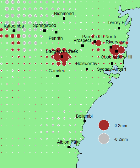
(a) MPRE;S12,D1
(b) MPRE;S12,D2
(c) MPRE;S15,D1
(d) MPRE;S15,D2
(e) MPRE;S12,D1 - MPRE;S12,D2
(f) MPRE;S12,D1 - MPRE;S15,D1
Figure 9: Bubble plots of the difference between the AWAP PRE estimates and the IDW1
PRE and the IDW2 PRE estimates using observations from 12 weather stations and from
15 weather stations.
42

---

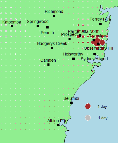
(a) MGT2MM;S12,D1
(b) MGT2MM;S12,D2
(c) MGT2MM;S15,D1
(d) MGT2MM;S15,D2
(e) MGT2MM;S12,D1 - MGT2MM;S12,D2
(f) MGT2MM;S12,D1 - MGT2MM;S15,D1
Figure 10: Bubble plots of the difference between the AWAP GT2MM estimates and the
IDW1 GT2MM and the IDW2 GT2MM estimates using observations from 12 weather
stations and from 15 weather stations.
43

---

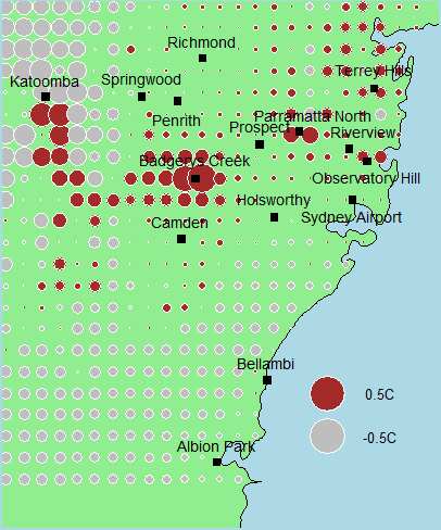
(a) MTMAX;S12,D1
(b) MTMAX;S12,D2
(c) MTMAX;S15,D1
(d) MTMAX;S15,D2
(e) MTMAX;S12,D1 - MTMAX;S12,D2
(f) MTMAX;S12,D1 - MTMAX;S15,D1
Figure 11: Bubble plots of the difference between the AWAP TMAX estimates and the
IDW1 TMAX and the IDW2 TMAX estimates using observations from 12 weather sta-
tions and from 15 weather stations.
44

---

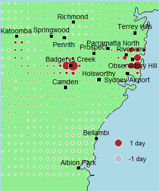
(a) MGT30C;S12,D1
(b) MGT30C;S12,D2
(c) MGT30C;S15,D1
(d) MGT30C;S15,D2
(e) MGT30C;S12,D1 - MGT30C;S12,D2
(f) MGT30C;S12,D1 - MGT30C;S15,D1
Figure 12: Bubble plots of the difference between the AWAP GT30C estimates and the
IDW1 GT30C and the IDW2 GT30C estimates using observations from 12 weather sta-
tions and from 15 weather stations.
45

---

Northwest of Katoomba, near Mt Victoria, and east of Katoomba, near Wentworth Falls,
the climate is similar to that of Katoomba and decreasing the weights of the Richmond,
Penrith weather stations improves the accuracy of weighted average estimates. However,
south of Katoomba in the Jamison Valley, the climate is quite different to that of Ka-
toomba and increasing the weights of Camden Airport, Penrith weather stations improves
the accuracy of weighted average estimates.
In general the inclusion of observations from additional weather stations moves the
IDW1 estimates closer to the AWAP estimates. For the three additional weather stations
chosen, the magnitude of the change tends to be less than that the magnitude of the
change between the IDW1 and IDW2 estimates and is often confined to regions close to
the additional weather stations. In Figure 9(f), the precipitation estimates are closer to
the AWAP estimates in regions close to each of the additional weather stations. However,
in Figure 11(f) there is a modest change in average maximum temperature estimates
across a wide area. Northwest of Katoomba, near Mt Victoria, there is a change away
from AWAP estimates arising from the inclusion, in particular, of observations from the
Badgerys Creek weather station.
For almost all of the Sydney Water area of operations, the average differences between
the IDW1 estimate using 12 weather stations and the AWAP estimate of:
• average daily precipitation per quarter is less than 0.6mm
• number of 2mm days per quarter is less than 5 days
• average maximum temperature per quarter is less than 1.2◦C
• number of 30◦C days per quarter is less than 4 days
Areas where the differences are greatest are:
• Blue mountains area between Katoomba and Springwood,
• The Illawarra, north of and inland from Bellambi, and the Royal National Park,
• The northern beaches and the Ku-ring-gai Chase National Park.
46

---

Some of these areas are lightly populated and so may have little impact on consumption
forecasts.
For most regions during the AMJ and JAS quarters, the values of GT30C weather
variable is close to zero and there is little difference between the IDW1 and AWAP esti-
mates.
The Sydney Water consumption model does not use the raw weather variable estimates
as explanatory variables, but rather the difference between those estimates and their long
term averages. It is possible that even if an estimate is inaccurate, so long as it is always
inaccurate by the same amount it still serves the model well. Studies on the accuracy of
AWAP data can be found in King et al. (2013) and Contractor et al. (2015).
7
Climate Extremes Indices
Included as explanatory variables in the SWCM are five weather variables used to cap-
ture the properties of the weather over the period of interest (Table 3). In this section,
we investigate some additional weather variables which also could have been used in the
SWCM. Some of the additional weather variables included in this investigation were taken
from the climate extremes indices defined by the Expert Team on Climate Change De-
tection and Indices (ETCCDI) and the Expert Team on Sector-specific Climate Indices
(ET-SCI), (ETCCDI (2017), ET-SCI (2017)). All of the ETCCDI and ET-SCI climate
extremes indices are functions of maximum, minimum temperature and/or precipitation,
none are functions of pan evaporation.
The heat wave indices, HWN, HWD and HWF are defined in Perkins and Alexander
(2012), where three different definitions of a heat wave were suggested. For this investiga-
tion, we use the definition based on the CTX90pct threshold. The CTX90pct threshold,
calculated for each calendar day, is the 90th percentile of maximum temperatures in a
15-day window centered on the day in question, over the period 1961-1990. A heat wave
occurs if this threshold is exceeded for three or more consecutive days.
Not all of the ETCCDI and ET-SCI climate extreme indices are relevant to the Sydney
region climate. For example, the ETCCDI index ID (Icing Days: Number of days when
47

---

the maximum temperature is less than 0◦C) is likely to be zero or very close to zero, almost
every year throughout the Sydney region. The climate extremes indices chosen for this
investigation are listed in Table 21. Each of the indices in Table 21 can be calculated either
monthly, quarterly or annually. Note that four of the five SWCM weather variables have
equivalent climate extreme indices included in Table 21: PRE is equivalent to PRCTOT;
GT2MM is equivalent to R2MM; TMAX is equivalent to TXM and GT30C is equivalent
to SU30.
To examine the relationship between climate extreme indices and water consumption,
we plotted the average actual and predicted consumption for single dwellings against
the climate extreme indices for over the period 2011/12 to 2015/16, (Figures 13 and
14 and Table 22). Single dwelling consumption tends to be more sensitive to weather
than consumption in other property types, due to the relatively larger outdoor water use
(gardens, pools, etc).
The climate extremes indices having the highest positive correlation with actual av-
erage single dwelling consumption are: TXM (0.981), SU28 (0.930), DTR (0.930), SU30
(0.905) and TX90P (0.890). The climate extremes indices having the highest negative cor-
relation with actual average single dwelling consumption are: TX10P (-0.986), R10MM
(-0.941), R20MM (-0.938), PRCTOT (-0.898) and R2MM (-0.892). The indices equiva-
lent to SWCM weather variables (PRCTOT, R2MM, TXM and SU30) are each strongly
correlated with the actual average single dwelling consumption. Other climate extremes
indicies are also strongly correlated with actual average single dwelling consumption and
may be worth considering for inclusion in any future release of the SWCM. Note that the
correlations listed above are calculated from only five pairs of data points and so are very
sensitive to changes in the data.
Wherever there is a strong correlation between a climate extreme index and the actual
average single dwelling consumption, there is also a strong correlation of the opposite sign
between the climate extreme index and the average single dwelling consumption prediction
error. This is consistent with the proposition that the SWCM tends to underestimate the
impact of weather on consumption, (Section 5.2).
48

---

Label
Description
FD
The number of days when the daily minimum temperature was < 0◦C.
SUn
The number days when the daily maximum temperature was > n◦C.
TXX
The maximum of the daily maximum temperatures.
TNX
The maximum of the daily minimum temperatures.
TXN
The minimum of the daily maximum temperatures.
TNN
The minimum of the daily minimum temperatures.
TXM
The mean of the daily maximum temperatures.
TNM
The mean of the daily minimum temperatures.
TR
The number of days when the daily minimum temperature was > 20◦C.
DTR
The mean of the differences between the daily maximum and daily
minimum temperatures.
TX10P
The number of days when the daily maximum temperature is less than
the 10th percentile of the 1961-1990 base period. A different percentile
is calculated for each month.
TN10P
The number of days when the daily minimum temperature is less than
the 10th percentile of the 1961-1990 base period. A different percentile
is calculated for each month.
TX90P
The number of days when the daily maximum temperature is greater
than the 90th percentile of the 1961-1990 base period. A different
percentile is calculated for each month.
TN90P
The number of days when the daily minimum temperature is greater
than the 90th percentile of the 1961-1990 base period. A different
percentile is calculated for each month.
HWN
The number of heat waves.
HWD
The length of the longest heat wave.
HWF
Number of heat wave days.
TX5Day
Maximum of average of maximum temperatures over a period of 5
consecutive days.
RX1Day
The maximum precipitation amount on a single day.
RX5Day
The maximum precipitation amount over a period of 5 consecutive days.
SDII
The average precipitation amount on days when the precipitation
amount was greater than 1 mm.
PRCTOT
The total precipitation.
CDD
The maximum number of consecutive days when the precipitation
amount of each day was less than 1 mm.
CWD
The maximum number of consecutive days when the precipitation
amount of each day was greater than 1 mm.
RnMM
The number of days when the precipitation amount was greater than n
mm.
Table 21: Climate extremes indices definitions.
49

---

Index
FY
Q1
Q2
Q3
Q4
SU25
0.890
0.422
0.724
0.927
0.700
SU28
0.930
0.744
0.807
0.923
0.879
SU30
0.905
0.756
0.837
0.878
0.765
SU32
0.859
0.499
0.784
0.880
0.809
TR
0.306
0.000
0.659
0.376
0.000
TXX
0.368
0.290
0.180
0.448
0.814
TNX
0.030
0.668
0.604
-0.367
0.363
TXN
0.538
0.641
0.452
0.814
-0.373
TNN
0.786
0.911
-0.274
0.735
-0.077
TXM
0.981
0.719
0.732
0.924
0.896
TNM
0.656
0.445
-0.083
0.818
0.956
TX10p
-0.986
-0.665
-0.652
-0.840
-0.781
TN10p
-0.714
-0.275
0.051
-0.748
-0.703
TX90p
0.890
0.559
0.885
0.823
0.952
TN90p
0.508
0.581
0.017
0.446
0.936
DTR
0.930
0.622
0.988
0.969
0.397
HWN
0.703
0.556
0.111
0.739
0.882
HWD
0.460
-0.087
0.420
0.857
0.417
HWF
0.658
0.372
0.003
0.805
0.708
TX5Day
0.841
0.515
0.470
0.912
0.715
RX1Day
-0.022
-0.330
-0.219
-0.063
0.348
RX5Day
-0.140
-0.492
-0.443
0.073
0.340
SDII
-0.623
-0.236
0.229
0.013
0.296
R1MM
-0.885
-0.593
-0.979
-0.903
-0.490
R2MM
-0.892
-0.542
-0.903
-0.899
-0.495
R5MM
-0.898
-0.613
-0.767
-0.886
-0.535
R10MM
-0.941
-0.501
-0.519
-0.778
-0.496
CDD
0.727
0.715
0.823
0.765
-0.163
CWD
-0.493
-0.503
-0.334
-0.733
-0.372
PRCTOT
-0.898
-0.551
-0.573
-0.776
-0.136
Table 22: Correlation of climate extreme indices and the average actual single dwelling
consumption. These correlations was calculated over the period 2011/12 to 2015/16 for
the entire financial year (FY) and for individual quarters Q1(JAS), Q2(OND), Q3(JFM)
and Q4(AMJ).
50

---

The correlation between climate extremes indices and average single dwelling con-
sumption was also calculated for individual quarters as well as for the entire financial
year, (22). For the high temperature quarters, Q2 and Q3, the climate extremes index
with the highest positive correlation was DTR, (0.988 and 0.969 respectively) and the
climate extremes index with the highest negative correlation was RX1MM, (-0.979 and
-0.903) respectively).
51

---

240
Actual
Predicted
240
Actual
Predicted
240
Actual
Predicted
230
230
230
220
220
220
Consumption (KL)
Consumption (KL)
Consumption (KL)
210
210
210
200
200
200
110
120
130
140
40
50
60
70
20
25
30
35
40
45
SU25
SU28
SU30
240
Actual
Predicted
240
Actual
Predicted
240
Actual
Predicted
230
230
230
220
220
220
Consumption (KL)
Consumption (KL)
Consumption (KL)
210
210
210
200
200
200
10
15
20
25
10
12
14
16
18
20
36
38
40
42
44
SU32
TR
TXX
240
Actual
Predicted
240
Actual
Predicted
240
Actual
Predicted
230
230
230
220
220
220
Consumption (KL)
Consumption (KL)
Consumption (KL)
210
210
210
200
200
200
21.2
21.4
21.6
21.8
22.0
22.2
22.4
11.5
12.0
12.5
13.0
13.5
1.5
2.0
2.5
TNX
TXN
TNN
240
Actual
Predicted
240
Actual
Predicted
240
Actual
Predicted
230
230
230
220
220
220
Consumption (KL)
Consumption (KL)
Consumption (KL)
210
210
210
200
200
200
22.0
22.5
23.0
23.5
11.8
12.0
12.2
12.4
12.6
4
5
6
7
8
9
10
11
TXM
TNM
TX10P
240
Actual
Predicted
240
Actual
Predicted
240
Actual
Predicted
230
230
230
220
220
220
Consumption (KL)
Consumption (KL)
Consumption (KL)
210
210
210
200
200
200
3
4
5
6
10
12
14
16
18
20
22
12
14
16
18
20
TN10P
TX90P
TN90P
Figure 13: Plot of average single dwelling actual and predicted consumption for the
financial years 2011/12 - 2015/16 as a function of the climate extremes indices SU25,
SU28, SU30, SU32, TR, TXX, TNX, TXN, TNN, TXM, TNM, TX10P, TN10P, TX90P
and TN90P calculated from AWAP data.
52

---

240
Actual
Predicted
240
Actual
Predicted
240
Actual
Predicted
230
230
230
220
220
220
Consumption (KL)
Consumption (KL)
Consumption (KL)
210
210
210
200
200
200
10.0
10.2
10.4
10.6
10.8
11.0
11.2
11.4
3
4
5
6
7
8
4
6
8
10
12
DTR
HWN
HWD
240
Actual
Predicted
240
Actual
Predicted
240
Actual
Predicted
230
230
230
220
220
220
Consumption (KL)
Consumption (KL)
Consumption (KL)
210
210
210
200
200
200
10
15
20
25
30
35
31.0
31.5
32.0
32.5
33.0
33.5
60
70
80
90
100
110
120
HWF
TX5Day
RX1Day
240
Actual
Predicted
240
Actual
Predicted
240
Actual
Predicted
230
230
230
220
220
220
Consumption (KL)
Consumption (KL)
Consumption (KL)
210
210
210
200
200
200
100
150
200
9.0
9.5
10.0
10.5
11.0
11.5
80
90
100
110
120
RX5Day
SDII
R1MM
240
Actual
Predicted
240
Actual
Predicted
240
Actual
Predicted
230
230
230
220
220
220
Consumption (KL)
Consumption (KL)
Consumption (KL)
210
210
210
200
200
200
65
70
75
80
85
90
95
40
45
50
55
60
65
20
25
30
35
40
R2MM
R5MM
R10MM
240
Actual
Predicted
240
Actual
Predicted
240
Actual
Predicted
230
230
230
220
220
220
Consumption (KL)
Consumption (KL)
Consumption (KL)
210
210
210
200
200
200
20
25
30
7
8
9
10
700
800
900
1000
1100
1200
1300
1400
CDD
CWD
PRCTOT
Figure 14: Plot of average single dwelling actual and predicted consumption for the
financial years 2011/12 - 2015/16 as a function of the climate extremes indices DTR,
HWN, HWD, HWF, TX5Day, RX1Day, RX5Day, SDII, R1MM, R2MM, R5MM, R10MM,
CDD, CWD and PRCTOT calculated from AWAP data.
53

---

8
Recommendations and Suggestions for Future Work
We make the following recommendations and suggestions for future work.
• Weather data at each property is estimated for the SWCM through the interpolation
of observations from 12 BoM weather stations. The accuracy of these estimations
may be improved through the inclusion of additional weather stations and/or the
choice of a better interpolation method. Alternatively, estimations could be taken
directly from a gridded data set such as AWAP.
• The NSW/ACT regional climate modelling project (NARCliM) is a regional climate
modelling project that has generated an ensemble of 12 future climate projections for
the region based on various global and regional climate models, (Evans et al. (2014)).
A set of weather scenarios, similar to those generated as part of this investigation,
could be generated from each of the NARCliM projections and be used to assess
the impact of the underlying model assumptions on consumption forecasts.
• The use of quarterly weather and consumption data may obscure the impact of
shorter term weather events on water consumption. Modelling of daily water con-
sumption may reveal additional significant relationships with weather and form the
basis for improved forecasts in the future.
• Sydney Water should consider a fundamental review of SWCM to examine the
model structure. This would enable other climate extremes indices to be examined
for their impact on water consumption.
54

---

Bibliography
Aalto, J., Pirinen, P., Heikkinen, J., and Venalainen, A. (2013). Spatial interpolation of
monthly climate data for Finland: comparing the performance of kriging and general-
ized additive models. Thoeretical and Applied Climatology, 112:99–111.
Abrams, B., Kumaradevan, S., Spanninks, F., and Sarafidis, V. (2012). An econometric
assessment of pricing Sydney’s residential water use. The Economic Record, 88:89–105.
Ailliot, P., Allard, D., Monbet, V., and Naveau, P. (2015). Stochastic weather generators:
an overview of weather type models. Journal of the French Statistical Society, 156:101–
113.
Brockwell, P. J. and Davis, R. A. (1991). Time series: theory and methods. Springer, 2nd
edition.
Contractor, S., Alexander, L. V., Donat, M. G., and Herold, N. (2015). How well do
gridded datasets of observed daily precipitation compare over Australia. Advances in
Meteorology, 2015.
Dobson, A. J. (2001). An introduction to generalized linear models. Chapman and Hall,
2nd edition.
ET-SCI (2017). Expert Team on Sector-specific Climate Indices. http://www.wmo.int/
pages/prog/wcp/ccl/opace/opace4/ET-SCI-4-1.php.
ETCCDI (2017). CCI/WRCP/JCOM Expert Team on Climate Change Detection and
Indices. https://www.wcrp-climate.org/etccdi.
Evans, J. P., Ji, F., Lee, C., Smith, P., Argueso, D., and Fita, L. (2014). Design of a
regional climate modelling projection ensemble experiment - NARCliM. Geoscientific
Model Development, 7:621–629.
Furrer, E. M. and Katz, R. W. (2007). Generalized linear modeling approach to stochastic
weather generators. Climate Research, 34:129–144.
55

---

Gregory, J. M., Wigley, T. M. L., and Jones, P. D. (1993). Application of Markov models
to area-average daily precipitation series and interannual variability in seasonal totals.
Climate Dynamics, 8:299–310.
Hastie, T. J. and Tibshirani, R. J. (1990). Generalized Additive Models. Chapman and
Hall.
Haylock, M. R., Hofstra, N., Tank, A. M. G. K., Klok, E. J., Jones, P. D., and New, M.
(2008). A European daily high-resolution gridded data set of surface temperature and
precipitation for 1950-2006. Journal of Geophysical Research, 113.
Hudson, G. and Wackernagel, H. (1994). Mapping temperature usinf kriging with external
drift: theory and an example from Scotland. International Journal of Climatology,
14:77–91.
Hutchinson, M. F. (1995). Interpolating mean rainfall using thin plate smoothing splines.
International Journal of Geographical Information Systems, 9:385–403.
IBM (2017).
IBM SPSS Statistics.
https://www.ibm.com/us-en/marketplace/
spss-statistics.
Jarvis, C. H. and Stuart, N. (2001). A comparison among strategies for interpolating max-
imum and minimum daily air temperatures. Part II: The interaction between number of
guiding variables and the type of interpolation method. Journal of Applied Meteorology,
40:1075–1084.
Jones, D. A., Wang, W., and Fawcett, R. (2009). High-quality spatial climate data-sets
for australia. Australian Meteorological and Oceanographic Journal, 58:233–248.
Jones, P. G. and Thornton, P. K. (1993). A rainfall generator for agricultural applications
in the tropics. Agricultural and Forest Meteorology, 63:1–19.
Katz, R. W. (1977). Precipitation as a chain-dependent process. Journal of Applied
Meteorology, 16:671–676.
56

---

Katz, R. W. and Parlange, M. B. (1995). Generalizations of chain-dependent processes:
application to hourly precipitation. Water Resources Research, 31:1331–1341.
King, A. D., Alexander, L. V., and Donat, M. G. (2013). The efficacy of using gridded data
to examine extreme rainfall characteristics: a case study for Australia. International
Journal of Climatology, 33:2376–2387.
Kysely, J. and Dubrovsky, M. (2005). Simulation of extreme temperature events by a
stochastic weater generator: effects of interdiurnal and interannual variablity reproduc-
tion. International Journal of Climatology, 25:251–269.
Mathworks (2017). The language of technical computing. https://au.mathworks.com/
products/matlab.html.
McCullagh, P. and Nelder, J. A. (1989). Generalized linear models. Chapman and Hall,
2nd edition.
Nalder, I. A. and Wein, R. W. (1998). Spatial interpolation of climatic normals: test
of a new method in the Canadian boreal forests. Agricultural and Forest Meteorology,
92:211–225.
Ninyerola, M., Pons, X., and Roure, J. M. (2000). A methodological approach of cli-
matological modelling of air temperature and precipitation through GIS techniques.
International Journal of Climatology, 20:1823–1841.
Perkins, S. E. and Alexander, L. V. (2012). On the measurement of heat waves. Journal
of Climate, 26.
Price, D. T., McKenney, D. W., Nelder, I. A., Hutchinson, M. F., and Kesteven, J. L.
(2000). A comparison of two statistical method for spatial interpolation of Canadian
monthly mean climate data. Agricultural and Forest Meteorology, 101:81–94.
Python (2017). Welcome to Python.org. https://www.python.org/.
R (2017). The R project for statistical computing. https://www.r-project.org/.
57

---

Richardson, C. W. (1981). Stochastic simulation of daily precipitation, temperature and
solar radiation. Water Resources Research, 17:182–190.
Rigby, B., Stasinopoulos, M., Heller, G., and Voudouris, V. (2014). The distribution
toolbox of GAMLSS. https://www.gamlss.org.
Rigby, R. A. and Stasinopoulos, D. M. (2005). Generalized additive models for location,
scale and shape. Journal of the Royal Statistical Society. Series C(Applied Statistics),
54:507–554.
Srikanthan, R. and McMahon, T. A. (2001). Stochastic generation of annual, monthy and
daily climate data: a review. Hydrology and Earth System Sciences, 5:653–670.
Stahl, K., Moore, R. D., Floyer, J. A., Asplin, M. G., and McKendry, I. G. (2006).
Comparison of approaches for spatial interpolation of daily air temperature in a large
region with complex topography and highly variable station density. Agricultural and
Forest Meteorology, 139:224–236.
Stein, M. L. (1999). Interpolation of Spatial Data: Some Theory for Kriging. Springer.
Suhaila, J. and Jemain, A. A. (2007). Fitting daily rainfall amount in Peninsular Malaysia
using several types of exponential distributions. Journal of Applied Sciences Research,
3:1027–1036.
Vicente-Serrano, S. M., Saz-Sanchez, M. A., and Cuadrat, J. M. (2003). Comparative
analysis of interpolation methods in the middle Ebro Valley (Spain): application to
annual precipitation and temperature. Climate Research, 24:161–180.
Wang, Q. J. and Nathan, R. J. (2007). A method for coupling daily and monthly time
scales in stochastic generation of rainfall series. Journal of Hydrology, 346:122–130.
Wilks, D. S. (1999). Interannual variability and extreme-value characteristics of several
stochastic daily precipitation models. Agricultural and Forest Meteorology, 93:153–169.
Wilks, D. S. and Wilby, R. L. (1999). The weather generation game: a review of stochastic
weather models. Progress in Physical Geography, 23:329–357.
58

---

Wood, S. N. (2006). Generalized Additive Models: An Introduction with R. Chapman and
Hall.
Wooldridge, J. M. (2010). Econometric Analysis of Cross Section and Panel Data. MIT
Press, 2nd edition.
59

---